Assessing Quantum Advantage through Random Circuit Sampling: Key Insights

**Introduction: Examining Quantum Advantage** As we venture deeper into the substantial claims surrounding quantum computing, the conversation often pivots to a pivotal question: Have we truly achieved quantum advantage? In this second installment of a three-part series, I’ll build upon our prior discussions about random circuit sampling (RCS) by scrutinizing the evidence that persuades me of its existence. **Evaluating Quantum Advantage** In assessing whether a quantum system offers a legitimate computational advantage, there are critical benchmarks we need to examine: 1. Does the experiment successfully tackle the intended computational challenge? 2. Does it provide a quantifiable advantage compared to traditional classical computations? 3. Is there a demonstrable practical benefit over the best classical algorithms? However, when we evaluate the RCS experiments, a significant complication arises. The early iterations of quantum computers used for these experiments were plagued by flaws and heavily influenced by error-inducing noise. This brings us to a pressing issue: how should we interpret results marred by this interference? In essence, we must confront two principal queries: - Even accounting for the noise, is random circuit sampling still fundamentally challenging for classical systems? - Can we assert, based purely on the experimental outputs, that we have effectively resolved the task posed? I believe we've accumulated a strong foundational understanding of these issues, which supports the assertion of quantum advantage. This understanding has emerged from an interdisciplinary approach, drawing on theoretical computer science, algorithm design, and physics over recent years. **Understanding Noisy Sampling Tasks** So, what precisely is the computational challenge addressed by these experiments? In an ideal RCS context, one starts with a random circuit, denoted as \(C\), which operates on \(n\) qubits. The goal is to sample from the output distribution derived from applying the circuit \(C\) on a specific reference state. The output probabilities follow the dictates of the Born rule upon measuring each qubit in a predetermined basis. What occurs on a noisy quantum computer during gate execution? It produces a compromised version, \(\rho_C\), of the intended state \(|C\rangle\), leading to sample outputs from this noisy distribution instead. The goal is assessing this task while factoring in the noise, which necessitates establishing a standard measure of accuracy in our noisy data preparation. A fitting approach is utilizing *fidelity*, a metric that quantifies the relationship between the ideal state and the noisy state. Fidelity is defined mathematically as follows: \[ F(C) = \langle C | \rho_C | C \rangle \] This value ranges from 1, indicating complete overlap with the ideal state, to 0, where orthogonality exists. Given this, we can define the computational task around sampling based on fixed fidelity levels in the noisy context. Importantly, achieving finite-fidelity RCS doesn’t require success for every possible circuit but rather mandates that the quantum device perform effectively on the majority of drawn circuits from the ensemble. When results are presented as a singular fidelity benchmark, they represent an average fidelity, denoted as \(F\). Current experiments claim to have effectively solved the finite-fidelity RCS problem with fidelity values near 0.1%. More compelling is the consistency of these results as circuit complexity scales, a factor critical to our later analysis. **The Complexity of Finite-Fidelity RCS** Let’s establish the stakes here: if quantum computations could be performed at highly accurate fidelity levels—say, around 90%—the case for a quantitative and practical advantage grows significantly stronger. Computational complexity theory strongly supports this position, as it parallels the evidence backing the complexity of problems like integer factoring and quantum system simulation. The intriguing aspect lies in how this classical durability diminishes as our fidelity level decreases. It's intuitive to think that lower fidelity, or \(\delta\), creates more favorable conditions for classical simulations. A larger deviation margin from the ideal state can make it easier for classical algorithms to approximate results. Counterintuitively, finite-fidelity RCS remains complex even at small values of \(\delta\). So far, there's no efficient classical algorithm that can successfully tackle—beyond trivial averages—the finite-fidelity tasks posed. The baseline, \(2^{-n}\)—indicating a completely mixed state without correlations—further emphasizes this challenge. While there are potential ways to improve efficiency in approaching near-ideal RCS by leaning on reduced fidelity, the required computational cost remains strictly exponential. The best-known classical approaches have arisen from research models simulating early experiments conducted by Google and USTC. **Scaling and Practicality in Quantum Experiments** The burning question now is: At which fidelity levels can we anticipate real-world advantages from RCS experiments? 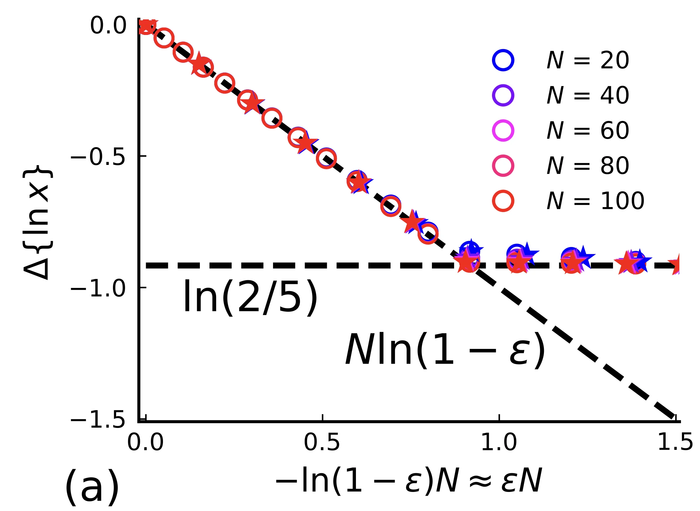To comprehend the scaling requirements, we visualize a noisy circuit operating on \(n\) qubits characterized by depth \(d\) and single-qubit noise strength \(\varepsilon\). Under this scenario, fidelity declines as follows: \[ F \sim \exp(-\varepsilon n d) \] For practical efficacy, fidelity must scale inversely with polynomial growth relative to \(n\). This implies that we require at least \(1/F^2\) samples to estimate average fidelity, rendering very small fidelities effectively undetectable experimentally. Connecting fidelity to near-ideal scenarios, where we ideally want \(\delta \geq 90\%\), grants an enhanced capability of yielding scalable advantages—a reasonable assumption moving forward. What’s critical is the architectural fidelity of the circuits and their parameter scaling in relation to the qubit count. The goal is to devise a noise profile that decreases as the qubit number rises while limiting circuity depth to only gradual increases. Realistically, the ideal scenario positions local noise rates to be less than a certain constant divided by \(n\), effectively maintaining circuit depth around logarithmic scaling with respect to the number of qubits involved. Maintaining fidelity at a level of \(F \gtrsim n^{-c}\) with a focus on scaling improvements motivated by engineering advancements suggests that while low-depth circuits might seem limiting, there can still be substantive advantages inherent in scenarios producing only \(\log(n)\) circuit depth. Ultimately, our analysis of fidelity versus the output benchmarks takes on a pivotal role, shedding light on the phase transitions experienced in evaluating the claims of quantum advantage and providing important insights for future experiments.

Understanding the Noise Threshold

The interplay between the noise in quantum systems and the performance of experiments hinges on a crucial element: a specific noise threshold represented by the constant \( c_A \). Below this value, when the local noise rate \( \varepsilon \) is less than \( c_A/n \), we observe that the cross-entropy benchmark (XEB) serves as a reliable estimate for average fidelity. This is particularly relevant because it defines the weak-noise regime where XEB metrics align closely with expected outcomes. However, when \( \varepsilon \) exceeds that threshold, we enter the strong-noise regime, where reliability diminishes—the XEB remains high even as fidelity plummets. To clarify the dynamics in play, during this weak-noise regime, the rate at which XEB decays as we deepen circuits is proportional to \( \varepsilon n \), indicating an exponential decay that can be mathematically expressed as \( \exp(-\varepsilon n d) \). In contrast, under strong noise conditions, the decay rates plateau, leading to a stark divergence between the high XEB values and the dwindling fidelity scores, which also decay as \( \exp(-\varepsilon n d) \) but irrespective of the noise scenarios at play.

Visualizing the Transition

The implications of these findings are captured in the accompanying plot which illustrates how the behavior of XEB relates to broader statistical mechanics principles. By leveraging this theoretical framework, researchers can extrapolate the noise thresholds pertinent to specific quantum architectures and circuit families. Essentially, this mapping serves not only illustrative purposes but also practical ones, highlighting how XEB performance varies significantly with noise levels and circuit depth. If this oscillation between reliable estimates and poor proxies strikes you as fundamental, it should. It reveals the intricacies implicit in experiments designed to measure quantum advantage. To claim success, experimental setups must definitively confirm their operations beneath the noise threshold, reinforcing their ability to approximate fidelity accurately.

Evaluating Experimental Robustness

As we analyze report findings on the nature of XEB in various experiments, it becomes apparent that the fidelity analysis operates not only on ideal conditions but must account for the realities of various noise profiles. For instance, both Google's experiment and those from USTC occupy positions below the crucial phase threshold, with Google’s initial trials flirting with the boundary. In this context, we should acknowledge that while these experiments reported XEB values consistently near 0.1%, they did so alongside improving error rates that outpaced the expected scalings typical for weak-noise dynamics. A deeper dive into the experimental framework reveals that assumptions made regarding local noise calibration could affect outcomes significantly. Experimenters often characterized noise at several levels—ranging from single gate assessments to broader circuit evaluations. This rigorous analysis demonstrates the critical need for a thorough understanding of noise effects on experimental fidelity since a significant portion of supplementary material underscores the process.

Importance of Accurate Proxies

The broad takeaway from this data is subtle yet significant: trusting the XEB as a fidelity estimator hinges on an intricate lattice of noise assessments and theoretical insights. Many real-world experiments are designed so that re-affirming noise characteristics allows researchers to apply the XEB as an effective proxy for fidelity, thereby addressing some skepticism regarding claims of quantum supremacy or advantage. Ultimately, parsing through the presented findings clarifies that experimental protocols aimed at decoding finite-fidelity random circuit sampling (RCS) grapple with unique challenges. The very methodologies employed to derive XEB and fidelity forms the basis for the legitimacy of claims regarding the efficiency of quantum systems. As such, maintaining a skeptical yet open-minded stance towards emerging data is critical for anyone navigating this rapidly evolving domain.

Closing Thoughts on Quantum Advantage

Understanding quantum advantage remains complex, especially when considering how experimental designs can shape outcomes. While current demonstrations aren't universally applicable across various devices, the ongoing evolution in this field mirrors what we’ve seen in earlier Bell tests. Those pioneering experiments, despite their limitations and loopholes, laid the groundwork for what we recognize as quantum mechanics today. Skepticism about the validity of quantum advantage stems largely from the need for ever more convoluted scenarios to explain its success. That's where the challenge lies: to refine our experimental methods until they require minimal assumptions about the devices used. This brings us to an interesting critique often raised: is it “unfair” to design tasks that inherently favor certain architectures? Indeed, the notion that tailored circuits can skew results casts a shadow on the objectivity of these tests. Yet framing this as a denial of quantum advantage misses the point. The tailored tasks may not transcend hardware limitations yet, but they still accomplish significant computational feats. Bridging the gap between hardware-specific solutions and more generalized applications is an essential step forward. The future of quantum advantage is poised to feature methodologies that enable efficient verification without relying on specific knowledge of test devices. This aspect isn’t just a nicety; it's a pathway to closing the gaps that still exist in our understanding of quantum computations. If you're involved in this field, this shift will be pivotal. Striving for tests that can validate outcomes based solely on measurement results is the frontier we need to explore. So as we look ahead, there's a dual challenge: advancing our experimental designs while also solidifying the theoretical frameworks that ground them. How researchers navigate this will determine the trajectory of quantum computing and its potential applications in the near future. The journey continues, and there's much at stake.